[Machine Learning] 월마트 선형회귀분석

선형회귀분석 - 중고차 가격에 영향을 미치는 요인 분석

1. 데이터셋 불러오기 및 확인

kaggle에서 제공하는 중고차 데이터셋을 불러옵니다.

여러 변수들의 전처리 과정을 거치고, 선형회귀분석을 통해 중고차 가격에 영향을 미치는 요인을 분석합니다.

데이터출처링크: Kaggle - Used Car Dataset

Used Car Dataset

Column	Description
car_name	모델명
registration_year	등록 날짜
insurance_validity	보험 유효성
fuel_type	연료 타입
seats	좌석 수
kms_driven	총 주행거리
ownership	소유권 형식
transmission	변속장치 타입
manufacturing_year	제작 년도
mileage(kmpl)	연비 (Kilometers per Liter)
engine(cc)	엔진 (cc)
max_power(bhp)	제동 마력 (Brake horse power = 실제 마력)
torque(Nm)	토크 (Newton meter) => 변수 삭제
price(in lakhs)	가격 (1 lakh = 100,000 루피)

import pandas as pd

origin = pd.read_csv("/Used Car Dataset.csv", index_col=0)

1-1 데이터 정보 확인

origin.info()

<class 'pandas.core.frame.DataFrame'>
Int64Index: 1553 entries, 0 to 1552
Data columns (total 14 columns):
 #   Column              Non-Null Count  Dtype
---  ------              --------------  -----
 0   car_name            1553 non-null   object
 1   registration_year   1553 non-null   object
 2   insurance_validity  1553 non-null   object
 3   fuel_type           1553 non-null   object
 4   seats               1553 non-null   int64
 5   kms_driven          1553 non-null   int64
 6   ownsership          1553 non-null   object
 7   transmission        1553 non-null   object
 8   manufacturing_year  1553 non-null   object
 9   mileage(kmpl)       1550 non-null   float64
 10  engine(cc)          1550 non-null   float64
 11  max_power(bhp)      1550 non-null   float64
 12  torque(Nm)          1549 non-null   float64
 13  price(in lakhs)     1553 non-null   float64
dtypes: float64(5), int64(2), object(7)
memory usage: 182.0+ KB

1-2 기술통계량 확인

• 기술통계량 확인 결과 정확하게 모든 값이 같은 변수가 있어서 제거 합니다.
• registration_year는 manufacturing_year와의 다중공선성을 고려하여 제거합니다.
• 제거할 변수: torque(Nm), registration_year

origin.describe(include="all").T

	count	unique	top	freq	mean	std	min	25%	50%	75%	max
car_name	1553	925	2017 BMW X1 sDrive20d Expedition	25	NaN	NaN	NaN	NaN	NaN	NaN	NaN
registration_year	1553	178	2017	40	NaN	NaN	NaN	NaN	NaN	NaN	NaN
insurance_validity	1553	6	Comprehensive	1084	NaN	NaN	NaN	NaN	NaN	NaN	NaN
fuel_type	1553	4	Petrol	1013	NaN	NaN	NaN	NaN	NaN	NaN	NaN
seats	1553.0	NaN	NaN	NaN	91.480361	2403.42406	4.0	5.0	5.0	5.0	67000.0
kms_driven	1553.0	NaN	NaN	NaN	52841.931101	40067.800347	620.0	30000.0	49134.0	70000.0	810000.0
ownsership	1553	22	First Owner	1240	NaN	NaN	NaN	NaN	NaN	NaN	NaN
transmission	1553	13	Manual	835	NaN	NaN	NaN	NaN	NaN	NaN	NaN
manufacturing_year	1553	19	2018	236	NaN	NaN	NaN	NaN	NaN	NaN	NaN
mileage(kmpl)	1550.0	NaN	NaN	NaN	236.927277	585.964295	7.81	16.3425	18.9	22.0	3996.0
engine(cc)	1550.0	NaN	NaN	NaN	14718574440.514194	218562947745.450348	5.0	1197.0	1462.0	1995.0	3258640000000.0
max_power(bhp)	1550.0	NaN	NaN	NaN	14718574440.514194	218562947745.450348	5.0	1197.0	1462.0	1995.0	3258640000000.0
torque(Nm)	1549.0	NaN	NaN	NaN	14239.891543	96662.407522	5.0	400.0	1173.0	8850.0	1464800.0
price(in lakhs)	1553.0	NaN	NaN	NaN	166.141494	3478.85509	1.0	4.66	7.14	17.0	95000.0

origin.drop(["max_power(bhp)", "registration_year"], axis=1, inplace=True)
origin.columns

Index(['car_name', 'insurance_validity', 'fuel_type', 'seats', 'kms_driven',
       'ownsership', 'transmission', 'manufacturing_year', 'mileage(kmpl)',
       'engine(cc)', 'torque(Nm)', 'price(in lakhs)'],
      dtype='object')

1-3 데이터 출력 상위 5개

origin.head(5)

	car_name	insurance_validity	fuel_type	seats	kms_driven	ownsership	transmission	manufacturing_year	mileage(kmpl)	engine(cc)	torque(Nm)	price(in lakhs)
0	2017 Mercedes-Benz S-Class S400	Comprehensive	Petrol	5	56000	First Owner	Automatic	2017	7.81	2996.0	333.0	63.75
1	2020 Nissan Magnite Turbo CVT XV Premium Opt BSVI	Comprehensive	Petrol	5	30615	First Owner	Automatic	2020	17.40	999.0	9863.0	8.99
2	2018 BMW X1 sDrive 20d xLine	Comprehensive	Diesel	5	24000	First Owner	Automatic	2018	20.68	1995.0	188.0	23.75
3	2019 Kia Seltos GTX Plus	Comprehensive	Petrol	5	18378	First Owner	Manual	2019	16.50	1353.0	13808.0	13.56
4	2019 Skoda Superb LK 1.8 TSI AT	Comprehensive	Petrol	5	44900	First Owner	Automatic	2019	14.67	1798.0	17746.0	24.00

1-4 결측치 확인

• 결측치의 갯수가 많지 않고 데이터 분석에 큰 영향을 미치지 않을 것으로 판단하여 제거 했습니다.

print(origin.isnull().sum())
origin.dropna(inplace=True)

car_name              0
insurance_validity    0
fuel_type             0
seats                 0
kms_driven            0
ownsership            0
transmission          0
manufacturing_year    0
mileage(kmpl)         3
engine(cc)            3
torque(Nm)            4
price(in lakhs)       0
dtype: int64

1-5 중복값 확인

• 다수의 중복된 중복된 값이 존재하였으므로 제거 합니다.

print(origin.duplicated().sum())
origin = origin.drop_duplicates(subset=origin.columns, ignore_index=True, keep="first")

420

1-6 변수명 변경

• torque 변수의 값들은 실제 bhp 변수의 값이므로 변수명 변경

origin.rename(
    columns={
        "ownsership": "ownership",
        "mileage(kmpl)": "mileage",
        "engine(cc)": "engine",
        "torque(Nm)": "bhp",
        "price(in lakhs)": "price",
    },
    inplace=True,
)

1-7 카테고리, 수치형 데이터 및 타겟 데이터 분류

• manufacturing_year

  • 시간에 따라 의존 변수가 선형적으로 변화하고 자동차의 가치가 매년 일정 비율로 감소한다고 가정하여, 년도를 수치형 변수로 사용하였습니다.

• seats

  • 좌석 수의 증가가 특정 변수(차량 가격)에 미치는지를 분석하기 위해 수치형 변수로 사용하였습니다.

categories = [
    "insurance_validity",
    "fuel_type",
    "ownership",
    "transmission",
]

num_features = [
    "kms_driven",
    "mileage",
    "engine",
    "bhp",
    "manufacturing_year",
    "seats",
]

target = "price"

2. 탐색적 데이터 분석 및 데이터 전처리

2-1 ownership 변수의 값 정리

• ownership 변수에 맞지 않는 여러 값들이 발견되어 정리 합니다.

origin = origin.loc[
    origin["ownership"].isin(["First Owner", "Second Owner", "Third Owner"])
]

2-2 명목형 변수와 수치형 변수 타입 지정

for category in categories:
    origin[category] = origin[category].astype("category")

origin["manufacturing_year"] = origin["manufacturing_year"].astype(int)

2-3 df변수에 1차 전처리된 origin 데이터 카피

df = origin.copy()
df.info()

<class 'pandas.core.frame.DataFrame'>
Int64Index: 1103 entries, 0 to 1128
Data columns (total 12 columns):
 #   Column              Non-Null Count  Dtype
---  ------              --------------  -----
 0   car_name            1103 non-null   object
 1   insurance_validity  1103 non-null   category
 2   fuel_type           1103 non-null   category
 3   seats               1103 non-null   int64
 4   kms_driven          1103 non-null   int64
 5   ownership           1103 non-null   category
 6   transmission        1103 non-null   category
 7   manufacturing_year  1103 non-null   int64
 8   mileage             1103 non-null   float64
 9   engine              1103 non-null   float64
 10  bhp                 1103 non-null   float64
 11  price               1103 non-null   float64
dtypes: category(4), float64(4), int64(3), object(1)
memory usage: 82.4+ KB

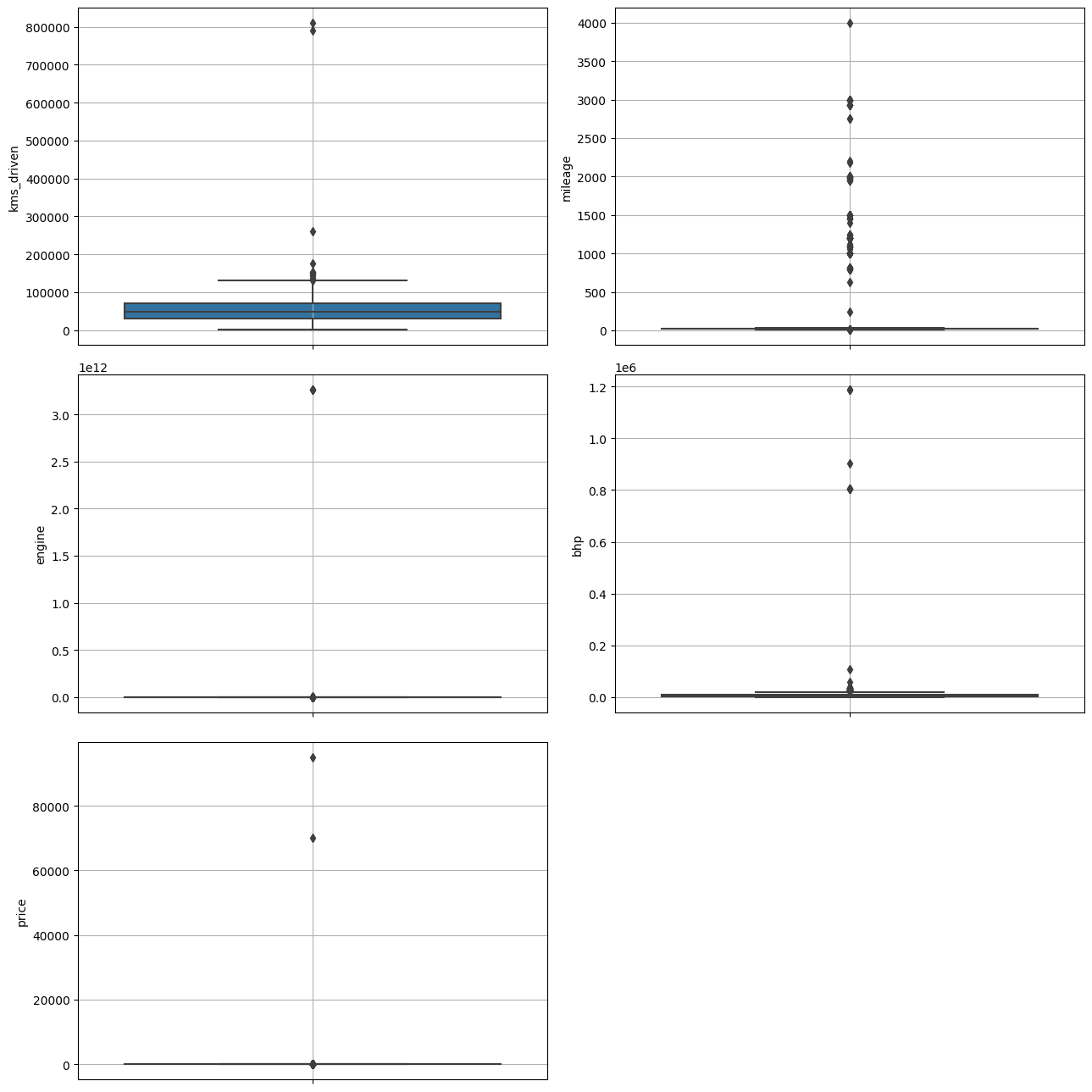
2-4 수치형 변수 boxplot 그래프로 이상치 확인

• engine, max_power, price 등에서 다수의 이상치가 관측 되었습니다.

import matplotlib.pyplot as plt
import seaborn as sns

features = ["kms_driven", "mileage", "engine", "bhp", "price"]
fig, axes = plt.subplots(3, 2, figsize=(13, 13), dpi=100)

for feature, ax in zip(features, axes.flatten()):
    sns.boxplot(data=df, y=feature, ax=ax)
    ax.grid(True)

fig.delaxes(axes[2, 1])

plt.tight_layout()
plt.show()
plt.close()

2-5. mileage(연비) 변수에 대한 이상치 확인 및 제거

• mileage값이 28.4에서 245.59로 급격하게 증가하는 이상치가 관측 되어 제거 합니다.

result = df.loc[df["mileage"] > 30, features].sort_values("mileage", ascending=False)
print(f"검색된 값: {result.shape[0]}")

df.drop(result.index, inplace=True)

검색된 값: 134

2-6. bhp(제동마력) 변수에 대한 이상치 확인 및 제거

• bhp의 단위가 이상할 정도로 큰 값들이 존재하여, 실제 차량 데이터와 비교해본 결과 실제 값으로 확인 되었고 단지 단위가 잘못 표기된 것으로 판단되어 전처리 과정을 거쳐 사용가능한 값으로 변환 하였습니다. (예 : 1186600 = 118.66)

• 2018 Mercedes-Benz S-Class Maybach S500 이상의 값들을 순차적으로 전처리 하였습니다.

thresholds = [460, 460, 600, 600]

for threshold in thresholds:
    df["bhp"] = df["bhp"].apply(lambda x: x / 10 if x > threshold else x)
    result = df.loc[df["bhp"] > threshold, features].sort_values("bhp", ascending=False)
    print(f"검색된 값: {result.shape[0]}")

검색된 값: 455
검색된 값: 11
검색된 값: 9
검색된 값: 0

2-7. price(가격) 변수에 대한 이상치 확인 및 제거

• 가격이 95000으로 기록된 이상치는 제거 합니다.

result = df.loc[df["price"] > 100, features].sort_values("price", ascending=False)
print(f"검색된 값: {result.shape[0]}")

result = df.loc[df["price"] > 100]
df.drop(result.index, inplace=True)

검색된 값: 1

2-7-1. 파생변수 생성하여 brand별 price 분포 확인

df["brand"] = df["car_name"].apply(lambda x: x.split(" ")[1])
df["brand"].unique()

array(['Mercedes-Benz', 'Nissan', 'BMW', 'Kia', 'Skoda', 'Honda',
       'Hyundai', 'Tata', 'Renault', 'Ford', 'Jeep', 'MG', 'Maruti',
       'Audi', 'Toyota', 'Jaguar', 'Volkswagen', 'Mahindra', 'Land',
       'Volvo', 'Isuzu', 'Mitsubishi', 'Porsche', 'Datsun', 'Lexus',
       'Mini', 'Fiat'], dtype=object)

plt.figure(figsize=(25, 10), dpi=200)
sns.boxplot(data=df, x="brand", y="price")
plt.grid()
plt.tight_layout()

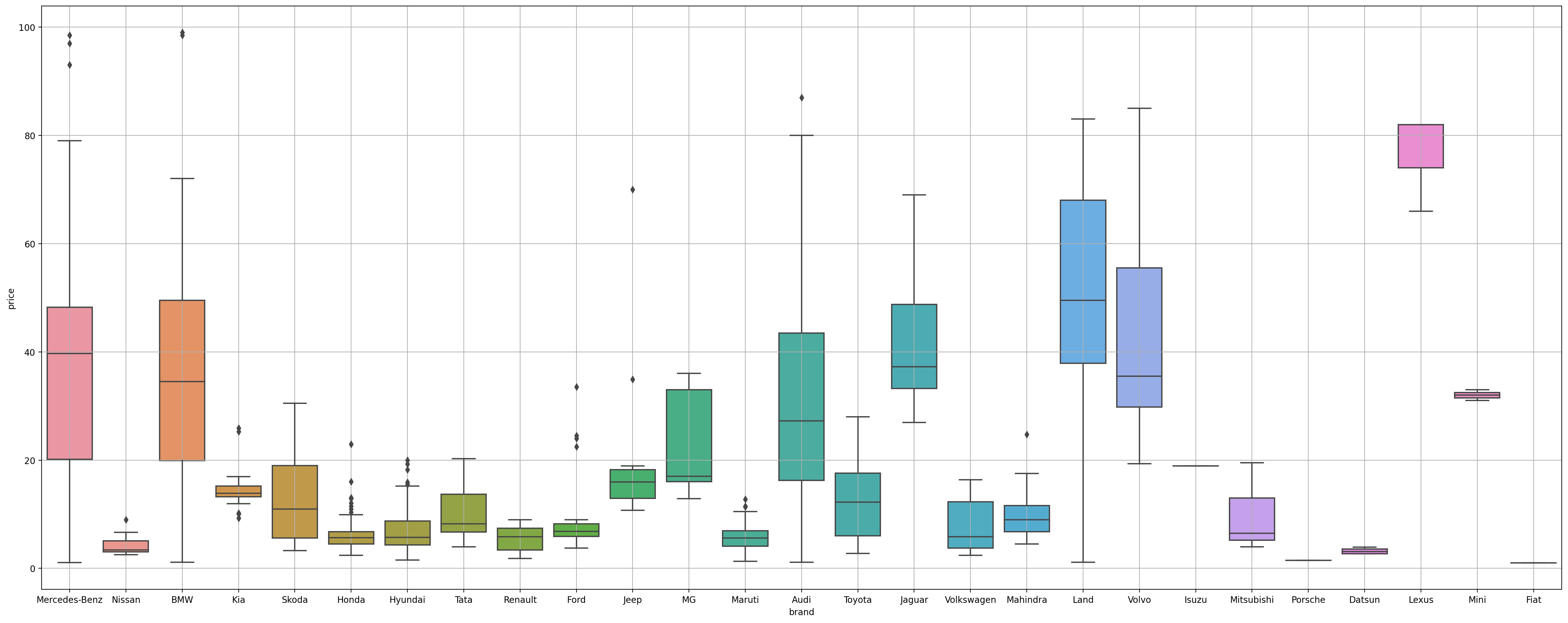
상위 5개 브랜드에서 가격이 비정상적으로 낮은(5 lakhs 이하) 데이터 제거 합니다.

result = df.loc[
    (
        (df["car_name"].str.contains("benz", case=False))
        | (df["car_name"].str.contains("bmw", case=False))
        | (df["car_name"].str.contains("audi", case=False))
        | (df["car_name"].str.contains("Land", case=False))
        | (df["car_name"].str.contains("Jaguar", case=False))
    )
    & (df["price"] < 5),
    ["car_name"] + num_features + [target],
].sort_values("price", ascending=False)

df.drop(result.index, inplace=True)

2-8. 자동차 브랜드별 평균 가격을 파생변수로 생성

df["car_name_mean_price"] = df.groupby("brand")["price"].transform("mean")

2-9. kms_driven(주행거리) 변수에 대한 이상치 확인

• 79만km와 81만km는 실제로 관측될 수 있는 수치이긴 하지만, 다른 차량 대비 지나치게 높은 값으로 결과의 신뢰성을 고려하여 이상치로 판단하고 제거 합니다.

df.drop(df[df["kms_driven"] > 700000].index, inplace=True)

2-10. engine(cc) 변수에 대한 이상치 확인 및 제거

df.loc[df["car_name"] == "2014 Mercedes-Benz S-Class S 500 L", "engine"] = 4663

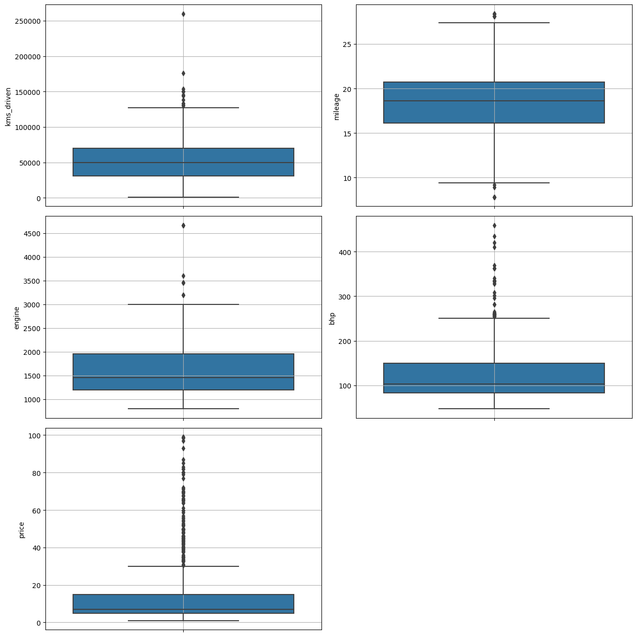
2-11. 수치형 변수 boxplot으로 이상치 재확인

features = ["kms_driven", "mileage", "engine", "bhp", "price"]
fig, axes = plt.subplots(3, 2, figsize=(13, 13), dpi=100)

for feature, ax in zip(features, axes.flatten()):
    sns.boxplot(data=df, y=feature, ax=ax)
    ax.grid(True)

fig.delaxes(axes[2, 1])

plt.tight_layout()
plt.show()
plt.close()

3. 선형회귀분석

num_features.pop(num_features.index("manufacturing_year"))

'manufacturing_year'

3-1. 히트맵 상관관계 확인

plt.figure(figsize=(10, 8), dpi=100)
sns.heatmap(
    df[num_features].join(df[target]).corr(),
    annot=True,
    cmap="coolwarm",
    fmt=".2f",
    annot_kws={"fontsize": 15},
)
plt.tight_layout()
plt.show()
plt.close()

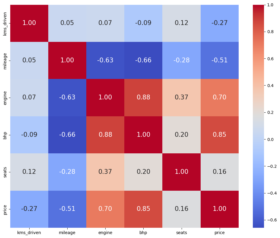
engine과 bhp에서 price와의 강한 양의 상관관계가 관측되었고, mileage와 price의 음의 상관관계가 관측되었습니다.

분석에 사용하지 않을 변수 제거

df.drop(["car_name", "brand"], axis=1, inplace=True)

카테고리 변수 확인

for i in categories:
    print(i, df[i].unique(), end="\n\n")
    print("=" * 100, end="\n\n")

insurance_validity ['Comprehensive', 'Third Party insurance', 'Zero Dep', 'Third Party']
Categories (4, object): ['Comprehensive', 'Third Party', 'Third Party insurance', 'Zero Dep']

====================================================================================================

fuel_type ['Petrol', 'Diesel', 'CNG']
Categories (3, object): ['CNG', 'Diesel', 'Petrol']

====================================================================================================

ownership ['First Owner', 'Second Owner', 'Third Owner']
Categories (3, object): ['First Owner', 'Second Owner', 'Third Owner']

====================================================================================================

transmission ['Automatic', 'Manual']
Categories (2, object): ['Automatic', 'Manual']

====================================================================================================

df.dtypes

insurance_validity     category
fuel_type              category
seats                     int64
kms_driven                int64
ownership              category
transmission           category
manufacturing_year        int64
mileage                 float64
engine                  float64
bhp                     float64
price                   float64
car_name_mean_price     float64
dtype: object

3-2. 카테고리 변수 더미화

df = pd.get_dummies(df, columns=categories, drop_first=True)

3-3. 수치형 변수 스케일링

from sklearn.preprocessing import StandardScaler

scaler = StandardScaler()

num_features_extended = num_features + ["manufacturing_year"] + ["car_name_mean_price"]

df[num_features_extended] = scaler.fit_transform(df[num_features_extended])

3-4. 데이터셋 분리

from sklearn.model_selection import train_test_split

x_train, x_test, y_train, y_test = train_test_split(
    df.drop(target, axis=1), df[target], test_size=0.2, random_state=42
)
x_train.shape, x_test.shape, y_train.shape, y_test.shape

((764, 15), (192, 15), (764,), (192,))

3-5. 다중공선성 확인 및 제거

VIF값이 10 이상인 변수를 제거 합니다

from statsmodels.stats.outliers_influence import variance_inflation_factor
from statsmodels.tools.tools import add_constant

df_with_const = add_constant(df)

vif = pd.DataFrame()
vif["Features"] = df_with_const.columns
vif["VIF"] = [
    variance_inflation_factor(df_with_const.values, i)
    for i in range(df_with_const.shape[1])
]

vif = (
    vif[vif["Features"] != "const"]
    .sort_values("VIF", ascending=False)
    .reset_index(drop=True)
)

vif[vif["VIF"] > 10]

	Features	VIF
0	fuel_type_Petrol	29.806683
1	fuel_type_Diesel	28.621752
2	bhp	10.949257

df.drop(["fuel_type_Petrol", "bhp"], axis=1, inplace=True)

3-6. 선형회귀분석

from sklearn.linear_model import LinearRegression

lr = LinearRegression()
lr.fit(x_train, y_train)

y_train_pred = lr.predict(x_train)
y_test_pred = lr.predict(x_test)

from sklearn.metrics import mean_squared_error, r2_score

print(f"Train RMSE: {mean_squared_error(y_train, y_train_pred):.2f}")
print(f"Test RMSE: {mean_squared_error(y_test, y_test_pred):.2f}")

print(f"Train R2: {r2_score(y_train, y_train_pred):.2f}")
print(f"Test R2: {r2_score(y_test, y_test_pred):.2f}")

Train RMSE: 46.44
Test RMSE: 58.93
Train R2: 0.83
Test R2: 0.82

많은 이상치와 중복데이터 그리고 결측치 등 데이터셋이 클린하지 않아서 전처리 과정에 많은 시간이 소요되었습니다.

그러나 선형회귀분석 결과는 Train RMSE: 46.44, Test RMSE: 58.93, Train R2: 0.83, Test R2: 0.82로 나쁘지 않은 결과를 보여줍니다.